If you want to capture the percentages of the employees attendance, you can use the Pivotable Attendance Report. This report has been flattened out so that you can use more spreadsheet operation on it such as generating a Pivot table of your employees attendance.

First, you need to extract the Pivotable Attendance Report. Click here to see how.

Once generated, you can import it to a Google Document if you want.

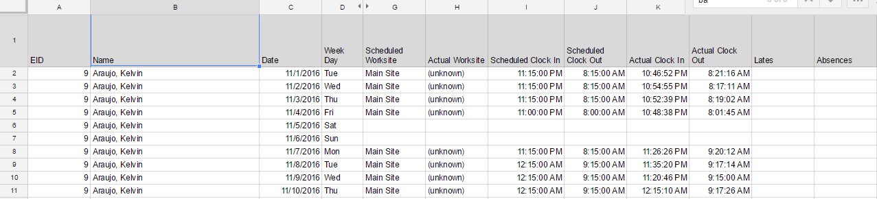
• Open the sheet
• Hide unnecessary columns if you want
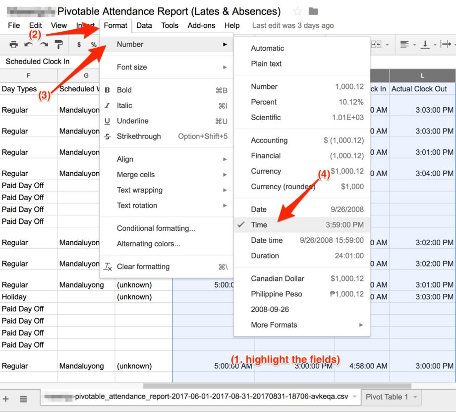
• Change the format of the columns Scheduled Clock In, Scheduled Clock Out, Actual Clock In and Actual Clock Out to TIME
  
  
• Insert 4 Columns after the Actual Clock Out column and name it Lates, Absences, Out Early & Perfect Attendance

Generate the Formulas

Lates

• For the LATES, select one cell under the Lates column then use this formula – “=If(Actual Clock In>Scheduled Clock In,1,0)”
• Hit Enter
• See screenshot for sample

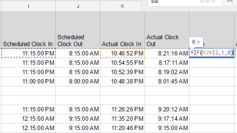
• Copy the cell and paste it for all cells under Lates column

Absences

• For the Absences, select one cell under the Absences column then use this formula – “=IF(AND(Scheduled Clock In>1,Scheduled Clock Out>1,Isblank(Actual Clock In),Isblank(Actual Clock Out)),1,0)“
• Hit Enter
• See screenshot for sample

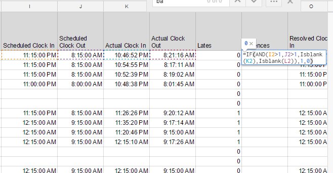
• Copy the cell and paste it for all cells under Absences column

Perfect Attendance

• For the Perfect Attendance, you need the get first the Out Early
  • Use this formula “=if(Actual Clock Out<Scheduled Clock Out,1,0)”
  • Click enter then copy for all cells under Out Early
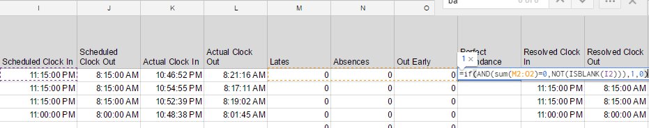
• Select one cell under the Perfect Attendance column then use this formula – “=if(AND(sum(Lates:Out Early)=0,NOT(ISBLANK(Scheduled Clock In))),1,0)“
• Hit Enter
• See screenshot for sample

• Copy the cell and paste it for all cells under Perfect Attendance column

Pivot the Data

• Select all Cells
• Under Data, choose Pivot Table
• A new sheet will be created named Pivot Table
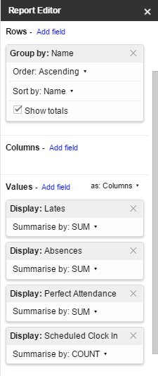
• On the Report Editor:
  • Rows – Add the field NAME
  • Values – Add the field LATES, ABSENCES, PERFECT ATTENDANCE & SCHEDULED CLOCK IN
  • For the Scheduled Clock In value – change the display to Summarise by: Count

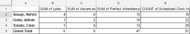
• Your Pivot Table would appear like this:

Add Percentages

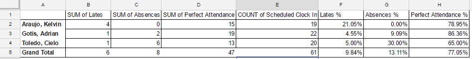
• Add 3 New Columns and name it “Lates Percentage”, “Absent Percentage” & “Perfect Attendance Percentage” or however you want to name it
• For the Lates %, use the formula “=Sum of Lates/Count of Scheduled Clock In” – (=B2/E2)
• For the Absences %, use the formula “Sum of Absences/Count of Scheduled Clock In” – (=C2/E2)
• For the Perfect Attendance %, use the formula “Sum of Perfect Attendance/Count of Scheduled Clock In – (=D2/E2)
• Change the format for those cells to Percent
• Your Pivot Table should look like this:

Now that’s how you figure out the Attendance Percentages of your employees using the Pivotable Attendance Report. If you have questions or suggestions, feel free to contact us at support@payrollhero.com.