If you want to capture the minutes or hours lates and absences of the employees attendance, you can use the Pivotable Attendance Report. This report has been flattened out so that you can use more spreadsheet operations on it such as generating a Pivot table of your employees attendance.

First, you need to extract the Pivotable Attendance Report. Click here to see how.

Once generated, you can import it to a Google Document if you want.

• Open the sheet
• Hide unnecessary columns if you want
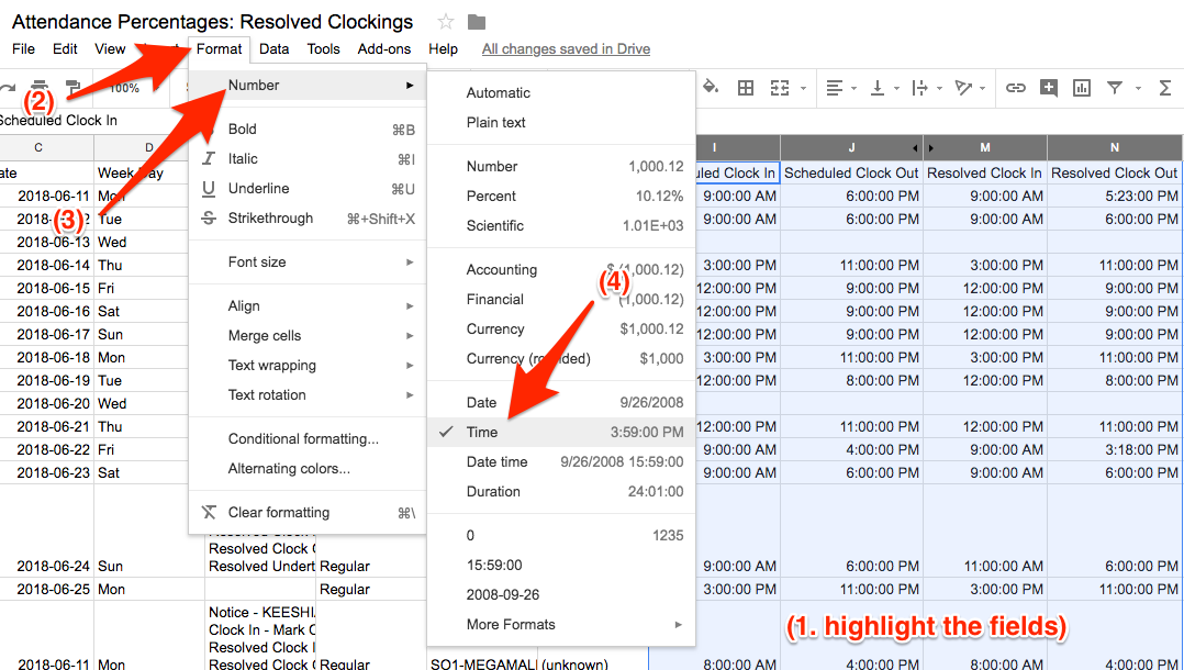
• Change the format of the columns “Scheduled Clock In, Scheduled Clock Out, Resolved Clock In and Resolved Clock Out” to TIME
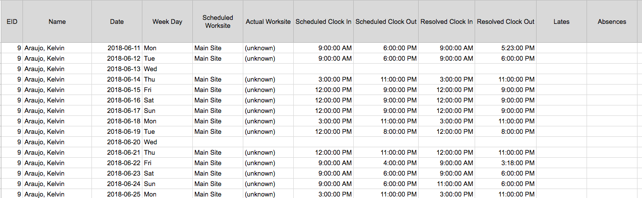
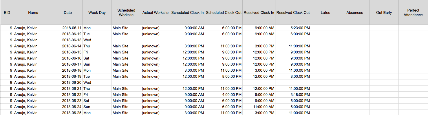
• Insert 2 Columns after the Resolved Clock Out column and name it Lates and Absences. See screenshot below.

Generate the Formulas

Lates

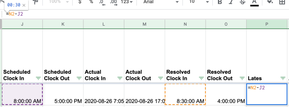
• For the LATES, select one cell under the Lates column
• And then deduct the “Resolved Clock In” to “Scheduled Clock In”
• Hit Enter
• See screenshot for sample
  
• Copy the cell and paste it for all cells under Lates column
• Note: There will be cases where in the employee is absent, and might show hours under their “Late” Column. You can simply delete this by filtering the “Resolved Clock in” Column. Here’s how:
  • Select all cells, then click “Data”
    
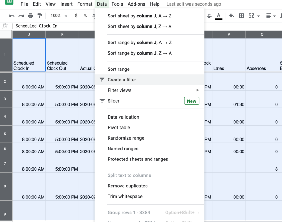
  • Click on ‘Create a filter’
  • Filter the “Resolved Clock In” column
    
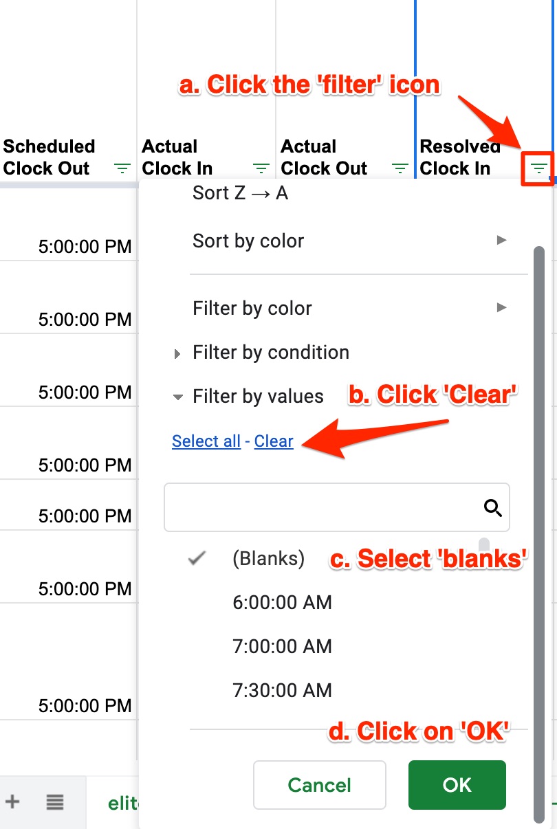
    • Click the ‘filter’ icon
    • Click ‘Clear’
    • Select “(Blanks)”
    • Click on OK
  • This will show all ‘lates’ with hours which you can just delete.
    
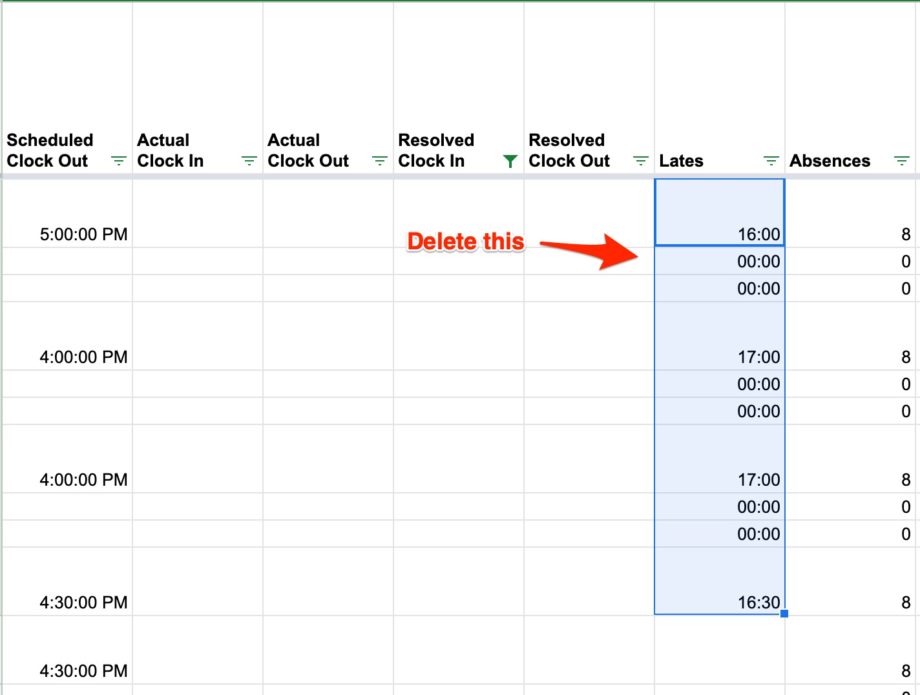
  • Remove the filter and that cleans up the “Late” column to only show the minutes and hours late of the employees.

Absences

• For the Absences, select one cell under the Absences column then use this formula below. Make sure to use the cell number on your spreadsheet for the Scheduled Clock In, Scheduled Clock Out, Resovlved Clock In and Scheduled Hours Less Unpaid Break:=IF(AND(Scheduled Clock In>1,Scheduled Clock Out>1,Isblank(Resolved Clock In),Isblank(Resolved Clock Out)),Scheduled Hours Less Unpaid Breaks,0)
• Hit Enter. See screenshot for sample 
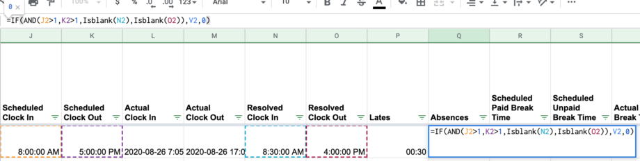
  • Scheduled Clock in is J2 cell number
  • Scheduled Clock out is K2
  • Resolved Clock in is N2
  • Resolved Clock out is O2
  • Scheduled Hours Less Unpaid Break is V2
• Copy the cell and paste it for all cells under Absences column

Pivot the Data

• Select all Cells
• Under Data, choose Pivot Table
• A new sheet will be created named Pivot Table
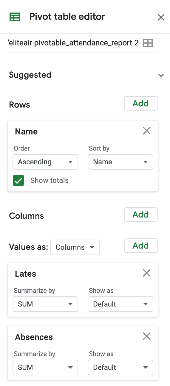
• On the Report Editor:
  • Rows – Add the field NAME
  • Values – Add the field LATES, ABSENCES
• It should look something like this:
  
• Your Pivot Table would appear like this:
  
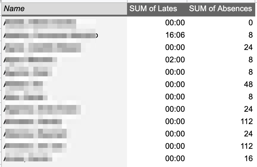
  • Note: SUM of Absences shows in hours.

If you have questions or suggestions, feel free to contact us at support@payrollhero.com.