We have had a few customers asking about how to extract night differential hours from the attendance report. ND is actually a function of our payroll calculator whereas attendance lives in Time, Attendance and Scheduling. We’ve put together a formula that would help you extract the ND hours from your pivotable attendance report.

I use google sheets for my spreadsheets. I’ve tried to write the instructions for any spreadsheet software but there may be differences.

Currently the scenarios this ND extractor covers is:

• Employee clock in before 6am but clock out before 9pm
• Employee clock out after 9pm
• Employee clock in after 9pm but clock out after 6am
• Employee clock in after 9pm but clocked out before 6am
• Employee clocks in before 9pm and clocks out before 6am
• Employee clocks in before 9pm and clocks out after 6am

Steps

Following these instructions is vital to this working correctly. You need to follow each step to get the desired result.

1. Generate the pivotable attendance report for the date period you require
2. Open the report in your spreadsheet software
3. Format columns I – N using HH:MM:SS (this is absolutely required)
   1. Click on format > number > time with matching format
4. Now insert 3 columns to the right of Column N
5. In cell O1 input: 06:00
6. In cell P1 input: 21:00
7. In cell Q1 input: ND
8. In cell O2 input: =iferror(SPLIT(M2, ” “))
   
9. In cell P2 input: =iferror(SPLIT(N2, ” “)) 
10. In cell Q2 input: =iferror(if(AND(O2<$O$1,O2>0,),$O$1–O2,if(P2>$P$1,P2–$P$1,IF(AND(O2>$P$1,P2<$O$1),N2–M2,IF(AND(O2<$P$1,P2>0,P2<$O$1),0.125+P2,if(AND(AND(O2<$P$1,O2>P2),P2<O2,P2>$O$1),value(“09:00”),))))))
    
11. Highlight cells O2, P2 and Q2 click on the bottom right corner and drag to fill all the cells below
    1. Potentially Required: If the spreadsheet is showing weird amounts like 0.375 in column Q you may need to adjust the formatting. Format column Q using HH:MM:SS
12. Now highlight the entire sheet
13. Click on Data > Pivot table
14. Select “Name” for the Rows
15. Select “ND” for the Value

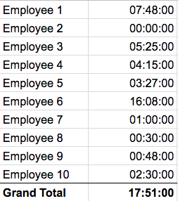
And your done! You should end up with a report that looks like:

If you have any additional questions or queries please don’t hesitate to contact support@payrollhero.com